Graph Representations for Predictive Modeling in Traffic Scenes

Abstract

Some deep reinforcement learning models are difficult to use in autonomous driving, as they require too much training time to learn useful and general control policies. This problem can be largely alleviated if the reinforcement learning agent has a meaningful representation of its surrounding environment. Representation learning is a set of techniques to achieve this goal. In this work, we develop a novel graph neural network and train it to reconstruct important information of the surrounding environment from the perspective of the ego agent. We further extract an encoded hidden state from the model which can be used as a meaningful representation of the surrounding environment for reinforcement learning agents.

Introduction

One of the most challenging tasks for Deep Reinforcement Learning (DRL) agents is learning accurate representations of their environment. This constitutes a limiting factor for DRL as it results in long training time for agents. Including state representation learning objectives into the reward function has been shown to improve representations and increase generalization ¹. Meaningful state representations are a cornerstone of accurate predictions in deep learning. Powerful representations encode relevant information and omit unnecessary details. Therefore, they reduce the complexity of following learning problems ² such as reinforcement learning.

Manual feature engineering is the most common approach to building representations. However, there are many techniques to let a neural network learn strong representations and eliminate the need for labor-intensive feature handcrafting. These techniques are grouped by the term representation learning.

We apply representation learning to the field of autonomous driving and more specifically traffic modeling. The behavior of agents is highly dependent on the surrounding traffic participants. The agents and their interaction in a driving scenario can be considered as a graph in which the nodes and edges represent the agents and their interaction respectively.

Graph Neural Networks (GNNs) are neural network architectures that are used for deep learning on graph-structured data ³. We use them for representation learning on traffic scenes. GNNs enable node-level, edge-level and graph-level predictions.

The remainder of this report is organized as follows: Section II introduces relevant concepts. In Section III we present our approach to building meaningful representations of traffic scenes and in Section IV we introduce our implementation. In Section V, we show our experiments. In Section VI we conclude our work and present ideas for further research.

Preliminaries

Graph Neural Networks

Traffic scenarios can be represented effectively using graphs. A graph \(G\) is a data structure that consists of a set of nodes (or vertices) \(V\) and a set of edges \(E\), i.e., \(G=(V,E)\). \(e_{ij}=(v_i,v_j) \in E\) denotes an edge pointing from \(v_j\) to \(v_i\), where \(v_i\in V\). \(N(v) = \{u\in V \mid (v,u)\in E\}\) denotes the neighborhood of a node \(v\). The node features \(\mathbf{h} \in \mathbf{R}^{n \times d}\) are defined as \(\mathbf{h} = \lbrace \vec{h}_i \mid i=1,...,n \rbrace\), where \(\vec{h}_i \in \mathbf{R}^d\) represents the feature vector of the node \(i\), \(n = \vert V \vert\) denotes the number of nodes and \(d\) denotes the dimension of the node feature vector. The edge features \(\mathbf{e} \in \mathbf{R}^{m \times c}\) are defined as \(\{\vec{e}_{ij} \mid i=1,...,n,j=1,...,N(i)\}\), where \(\vec{e}_{ij} \in \mathbf{R}^{c}\) represent the feature vector of the edge \((i,j)\), \(m = \vert E \vert\) denotes the number of edges and \(c\) denotes the dimension of the edge feature vector.

GNN uses a form of neural message passing (MPNN) to learn graph-structured data. MPNN treats graph convolutions as a message passing process in which vector messages can be passed from one node to another along edges directly. MPNN runs \(L\) step message passing iterations to let messages propagate further⁴. The message passing function at message passing step \(l\) is defined as \(\vec{h}^{l}_i = f_n(\vec{h}^{l-1}_i,m^{l}_i)\), where \(m^{l}_i = \Phi(\{\vec{e}^{\,l}_{ij}\}_{j\in N(i)})\), \(\vec{e}^{\,l}_{ij} = f_e(\vec{h}^{l-1}_i,\vec{h}^{l-1}_j,\vec{e}^{\, l-1}_{ij})\). \(m^{l}_i\) represents the message of node \(i\) at message passing step \(l\), \(\Phi\) denotes an aggregation operation, \(f_n\) and \(f_e\) are functions with learnable parameters.

Edge Convolution

The edge convolution (Edge Conv) ⁵ we use is an asymmetric edge function. It operates the edges connecting neighboring pairs of nodes. Specifically, it updates the target node features by \(\ref{eq:1}\). The operation captures the hidden information from the target node feature \(\vec{h}_i\) and also the neighborhood information, captured by \(\vec{h}_j-\vec{h}_i\).

\[\begin{equation}\tag{Eq. 1}\label{eq:1} \quad \vec{h}_i' =\max_{j \in \mathcal N_i}\text{MLP}_{\theta}([\vec{h}_i,\vec{h}_j-\vec{h}_i]) \end{equation}\]

The concatenated vector \([\vec{h}_i,\vec{h}_j-\vec{h}_i]\) is transformed by a Multilayer perceptron (MLP) and then aggregated by a max operation.

Edge-Featured Graph Attention Network

Edge-Featured Graph Attention Networks (EGAT) ⁶ are an extension of Graph Attention Neural Networks (GAT) ⁷. Compared to GATs, EGATs allow for implicitly assigning different importances to different neighbor nodes, considering not only node features but also edge features. They don’t depend on knowing the entire graph structure upfront. Additionally, EGAT is computationally efficient. It does not require costly matrix operations. We use the node attention block of EGAT layer in our experiment. A node attention block of EGAT layer takes both node features \(\mathbf{h}\) and edge features \(\mathbf{e}\) as input and produces a new set of node features \(\mathbf{h}'\) as output, where \(\mathbf{h}'=\{\vec{h}_i' \mid i=1,...,n\}\).

Node and edge feature transformation

First, the node features \(\mathbf{h}\) and edge features \(\mathbf{e}\) are transformed by a linear layer,

\[\begin{equation}\tag{Eq. 2}\label{eq:2} \quad \mathbf{h}^* = \mathbf{W}_{h}\cdot\mathbf{h} \end{equation}\]

\[\begin{equation}\tag{Eq. 3}\label{eq:3} \quad \mathbf{e}^* = \mathbf{W}_{e}\cdot\mathbf{e} \end{equation}\]

where \(\mathbf{h}^*\) and \(\mathbf{e}^*\) are the projected node features and edge features respectively.

Edge enhanced attention

Given a target node \(i\), the attention coefficient \(\alpha_{i,j}\) is calculated by \(\ref{eq:4}\), \(\alpha_{i,j}\) indicates the importance of the node \(j\) to node \(i\) jointly considering node and edge features.

\[\begin{equation}\tag{Eq. 4}\label{eq:4} \quad \alpha_{i,j}=\frac{\exp(\text{LeakyReLu}(\mathbf{a}^\mathrm{T}[\vec{h}_i^{*} \Vert \vec{h}_j^{*} \Vert \vec{e}_{ij}^*]))}{\sum_{k \in N(i)}\exp(\text{LeakyReLu}(\mathbf{a}^\mathrm{T}[\vec{h}^*_{i} \Vert \vec{h}^*_{j} \Vert \vec{e}^*_{ij}]))} \end{equation}\]

Here, \(\mathbf{a}\) is a linear layer and \(N(i)\) is the neighbor nodes of node i in the graph. The node feature \(\vec{h}^{'}_{i}\) is then updated by calculating a weighted sum of edge-integrated node features over its neighbor nodes, followed by a sigmoid function.

\[\begin{equation}\tag{Eq. 5}\label{eq:5} \quad \vec{h}'_{i}=\sigma\left(\sum_{j\in N(i)}\alpha_{ij}\mathbf{W}_h^\mathrm{T}[\vec{e}^*_{ij} \Vert \vec{h^*_{j}}]\right) \end{equation}\]

Similar to GAT, we apply multi-head attention and run several independent attention mechanisms to get a stable self-attention mechanism output. Additionally, it allows the model to jointly attend to the information from different representation sub-spaces at different positions. The output of each attention head is concatenated as the final updated node feature \(\vec{h}^{+}_{i}\).

\[\begin{equation}\tag{Eq. 6}\label{eq:6} \quad \vec{h}^{+}_{i}=\mathop{\Vert}\limits_{k=1}^{K}\vec{h}^{k'}_{i} \end{equation}\]

Here, \(K\) is the number of attention heads and \(\mathop{\Vert}\) indicates the concatenation operation.

Methodology

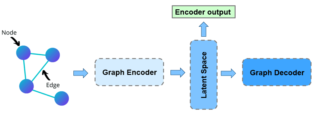
In this section, we introduce the approach of constructing the graph data from the highD dataset and describe the definition of maximum closeness which is the ground truth label for reconstruction. We elaborate our reconstruction neural network and the loss function we used in the training process. Successful reconstruction of the important information of the agent environment indicates that the model is able to extract the latent information from the surrounding environment. Thus, we can extract an encoder output from the model and use it as a meaningful representation of the surrounding environment for reinforcement learning. Fig. 1 illustrates the basic concept of extracting the encoder output from the model pipeline.

Encoder output extraction

Graph extraction

The basis of our GNN training data is the highD dataset ⁸, a dataset of vehicle trajectories on highways. We extract fully connected graphs from highD. In our training dataset, graph nodes represent traffic participants and edges represent the relationship between different traffic participants. For node \(i\), the position \((x_i, y_i)\) acts as the node feature \(\vec{h}_i\). The edge feature \(\vec{e}_{ij}\) for the edge between node \(i\) and node \(j\) consists of the Euclidean distance \(d_{ij}\) \(\ref{eq:7}\), sine of the relative angle \(\sin(\alpha_{ij})\) \(\ref{eq:8}\) and cosine of the relative angle \(\cos(\alpha_{ij})\) \(\ref{eq:9}\).

\[\begin{equation}\tag{Eq. 7}\label{eq:7} \quad d_{ij} = \sqrt{(x_i-x_j)^2+(y_i-y_j)^2} \end{equation}\]

\[\begin{equation}\tag{Eq. 8}\label{eq:8} \quad \sin\alpha_{ij} = \frac{y_i-y_j}{d_{ij}} \end{equation}\]

\[\begin{equation}\tag{Eq. 9}\label{eq:9} \quad \cos\alpha_{ij} = \frac{x_i-x_j}{d_{ij}} \end{equation}\]

Thus, our constructed graph consists of the node feature vector \(\mathbf{h}\) \(\ref{eq:12}\) and the edge feature vector \(\mathbf{e}\) \(\ref{eq:13}\).

\[\begin{equation}\tag{Eq. 10}\label{eq:10} \quad \vec{h}_i = [x_i, y_i] \end{equation}\]

\[\begin{equation}\tag{Eq. 11}\label{eq:11} \quad \vec{e}_{ij} = [d_{ij}, \sin(\alpha_{ij}), \cos(\alpha_{ij})] \end{equation}\]

\[\begin{equation}\tag{Eq. 12}\label{eq:12} \quad \mathbf{h} = \{\vec{h}_i \mid i=1,...,N\} \end{equation}\]

\[\begin{equation}\tag{Eq. 13}\label{eq:13} \quad \mathbf{e} = \{\vec{e}_{ij} \mid i=1,...,N,j=1,...,N_i\} \end{equation}\]

Maximum closeness

We divide the area surrounding the ego agent into eight \(45^{\circ}\) segments \(\mathbf{R} = \{R_{i} \mid i=1,...,8\}\) as illustrated in Fig. 2, referred to as angular regions in the following.

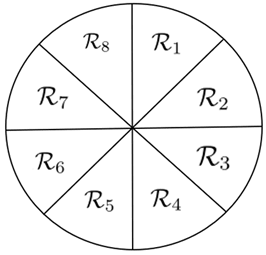
We define closeness \(c_{i,j} \in [0,1]\) \(\ref{eq:14}\) as our proximity measure between the node \(i\) (ego agent) and node \(j\) (other traffic participants). Unlike the euclidean distance, closeness provides a smooth label and prevents discontinuities resulting from empty regions. \(c_{i,j}\) is \(0\) for all values greater than or equal to \(D_{max}\) and \(1\) if the euclidean distance \(d_{i,j}\) is \(0\). The maximum closeness of node \(i\) in angular region \(m\) is defined as \({c}^{+}_{i,m}\) \(\ref{eq:15}\). Our ground truth label, \(\mathbf{c}^{+}\) \(\ref{eq:16}\), is the vector of the maximum closenesses.

\[\begin{equation}\tag{Eq. 14}\label{eq:14} \quad c_{i,j} = 1 - \frac{\min(d_{i,j},D_{max})}{D_{max}} \end{equation}\]

\[\begin{equation}\tag{Eq. 15}\label{eq:15} \quad c^{+}_{i,m} = \max_{j \in \mathcal{R}_m}\{c_{ij}\} \end{equation}\]

\[\begin{equation}\tag{Eq. 16}\label{eq:16} \quad \mathbf{c}^{+} = \{c^{+}_{i,m} \mid i=1,...,N,m=1,...,8\} \end{equation}\]

Model

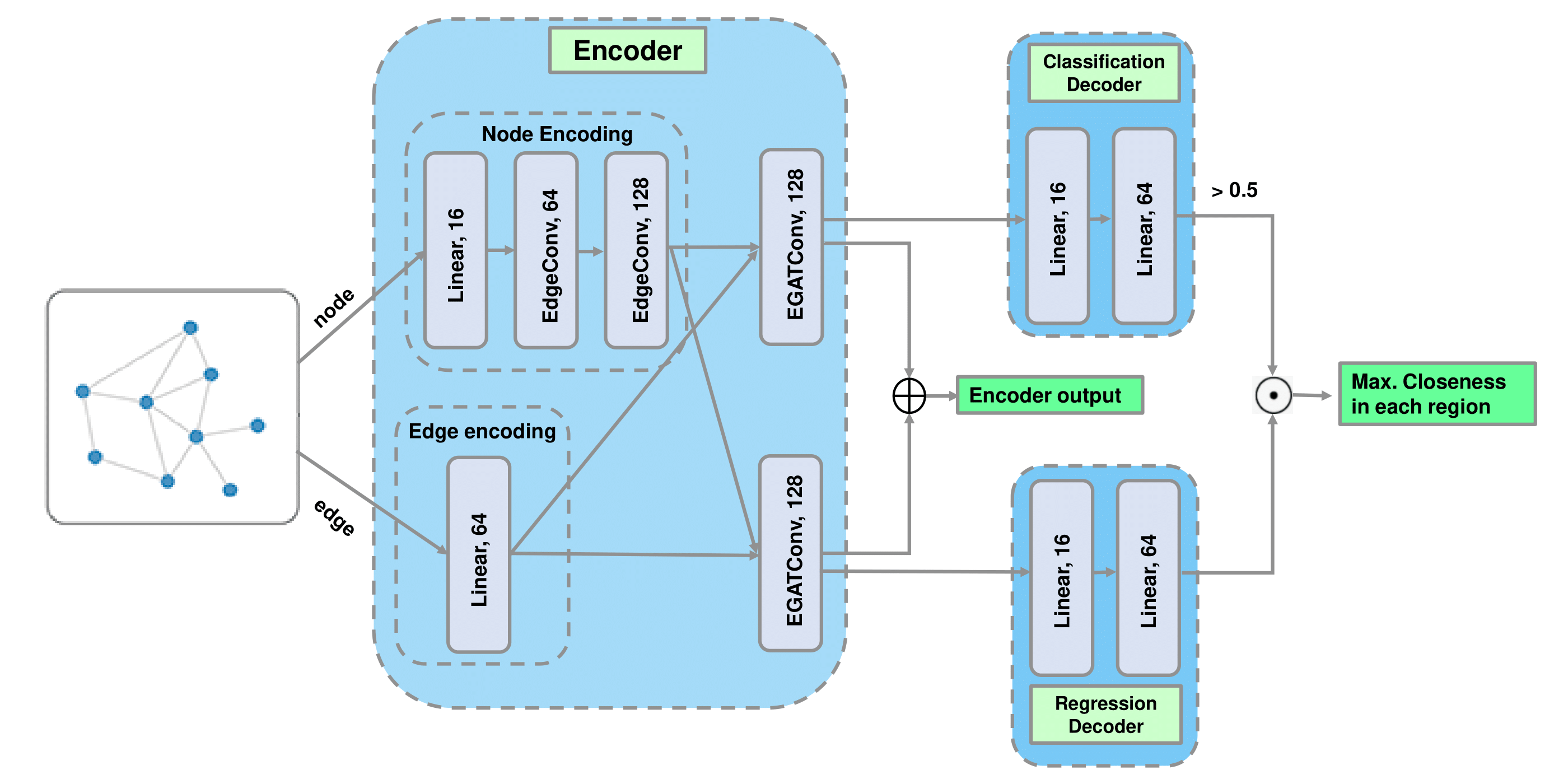
We describe our general pipeline in Fig. 3 We construct a fully connected graph to represent the agent environment. Our model takes the fully connected graph, i.e., all node feature vectors \(\mathbf{h}\) and edge feature vectors \(\mathbf{e}\) as inputs and outputs the maximum closeness of each target node in the eight regions, i.e., \(\mathbf{c}^{+}\). Additionally, we extract the output of the encoder which can be used as the input for reinforcement learning.

“Fig. 3: Model architecture”

Classifier and regressor

We divide this maximum closeness reconstruction task into a binary classification task and a regression task. We train a classifier to predict the existence of agents in each region. Simultaneously, we train a regressor to reconstruct the maximum closeness in the regions in which agents exist. The final output is then calculated as the element-wise multiplication of classification output and regression output.

Encoding graph information

Each node attribute has two features: \(x_i\) and \(y_i\) position. Each edge attribute has three features: relative distance \(d_{ij}\), sine of relative angle \(\sin(\alpha_{ij})\) and cosine of relative angle \(\cos(\alpha_{ij})\). Thus the node input and edge input has shape \((n,2)\) and \((m,3)\) respectively, where \(n\) is the number of nodes and \(m\) is the number of edges.

We use a linear layer followed by two Edge Conv layers to process node input and obtain a \((n,128)\) tensor: \(E_{node}\). Similarly, we use a linear layer to process edge input and get a \((m,64)\) tensor: \(E_{edge}\).

Extracting encoder output

We use two node attention blocks of EGAT to aggregate \(E_{node}\) and \(E_{edge}\) for the classifier and regressor separately, so to obtain a \((n,128)\) tensor: \(E_{cls}\) and a \((n,128)\) tensor: \(E_{reg}\). The encoder output \(E_{encoder}\) is defined as the concatenation of \(E_{cls}\) and \(E_{reg}\).

Decoding graph information

We use two linear layers as the classification decoder and regression decoder. The activation function of the last layer in both decoders is a sigmoid function, so we obtain an output value between \(0\) and \(1\). Then, the classification output is set to \(1\) if its value is greater than \(0.5\) and \(0\) otherwise. The model output is calculated as regression output element multiplied by classification output.

Loss function

This model is trained with a classification loss \(\mathcal{L}_{cls}\) and a regression loss \(\mathcal{L}_{reg}\). The total loss is calculated in \(\ref{eq:17}\), where the design parameter \(\beta\) allows to balance the weight of the regression loss in relation to the classification loss.

\[\begin{equation}\tag{Eq. 17}\label{eq:17} \quad \mathcal{L}=\beta\mathcal{L}_{reg} + \mathcal{L}_{cls} \end{equation}\]

Implementation

Our implementation uses the CommonRoad-Geometric package developed at the chair of Robotics, Artificial Intelligence and Embedded Systems at the Technical University of Munich (TUM). CommonRoad-Geometric is a geometric deep learning library for autonomous driving that we use to extract graph data from traffic scenarios. It is built on top of PyTorch Geometric ⁹ and the CommonRoad framework ¹⁰. CommonRoad is a collection of benchmarks for autonomous driving that enable reproducibility and PyTorch Geometric is a popular PyTorch ¹¹ based library for deep learning on graphs. As explained in Subsection [3.1], we use highD as the basis of our training data.

Extraction implementation

Model implementation

Visualization implementation

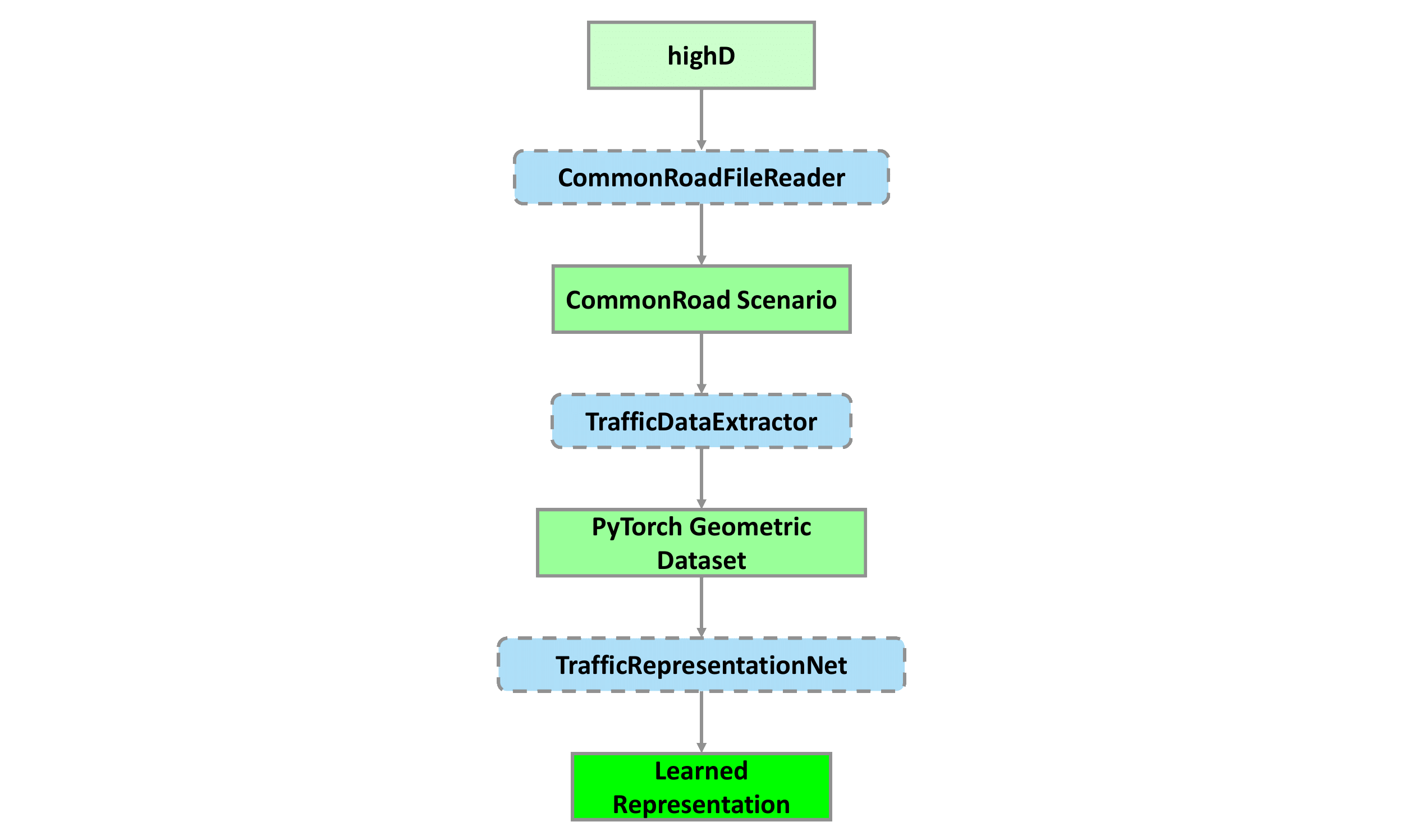
Our package traffic_scene_representation is split into three subpackages: extraction, model and visualization (see Fig. 4). The extraction package contains two classes: extractor which extends the CommonRoad Geometric class StandardTrafficExtractor and collector which extends the CommonRoad Geometric class BaseDatasetCollector. extractor is responsible for extracting one PyTorch Geometric graph data object from a single scenario and timestep as described in Subsection 3.1. The class collector is responsible for collecting the entire training and test dataset from the highD dataset and saving the files to the disk. Furthermore, we built a GNN model as described in 3.3 using PyTorch Geometric. For building the GNN model, we implement three neural network layers, namely the classes EGATConvs, EdgeConv and MLP. The entire model is implemented in the class TrafficRepresentationNet. Additionally, we provide the tools to perform PCA decomposition on all encoder outputs. We also provide a simple set of visualization scripts, combined in the subpackage visualization, that can render the different traffic participants, the lanes and the prediction results. It can also visualize the PCA decomposition heatmap. This is useful for debugging and showcasing purposes. It is written using the Python libraries Pillow, a popular Python library for image manipulation and matplotlib, a commonly use plotting library.

Experiments

Training details

We use our constructed PyTorch Geometric graph dataset in our experiment. It contains \(80000\) training samples, \(10000\) validation samples and \(10000\) test samples. We train our models for \(50\) epochs with batch size \(64\), using the Adam optimizer initialized with a learning rate of \(0.001\) and exponential decay rate of \(0.9\). All Edge Conv layers and EGAT layers are followed by BatchNormalization and ReLU activation. All linear layers except the last linear layer in both decoders are followed with ReLU activation. The classification loss \(\mathcal{L}_{cls}\) is binary cross-entropy loss and the regression loss \(\mathcal{L}_{reg}\) is Huber loss. We set the hyperparameter \(\beta\) in loss function to \(100\).

Converged losses of the model by using different encoder output dimensions

Reconstruction performance by using different encoder dimensions

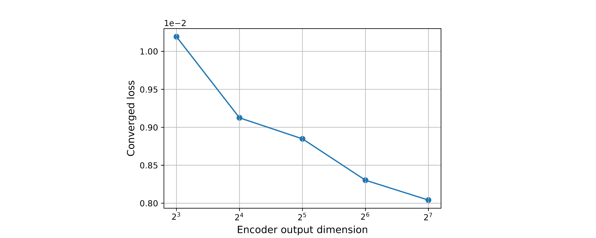
We set up experiments for testing the performance of model using different encoder dimensions. We set the feature dimension of \(E_{cls}\) and \(E_{reg}\) to \(8\), \(16\), \(32\), \(64\), \(128\) in five experiments respectively, simultaneously, modify the input dimension of the following linear layer to the same dimension and keep other hyperparameters unchanged. The converged loss of each encoder dimension is illustrated in Fig. 5. We can see that models with higher number of dimensions in the encoder output archive a lower converged loss than models with few dimensions.

Additionally, we observe that even using an encoder dimension of \(8\), the model still performs very well. It indicates that we can use a low-dimensional encoder output to represent the agent environment and that we can use it as the input for reinforcement learning agents.

Reconstruction result and interpretation of the learned representations

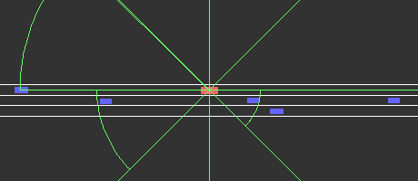
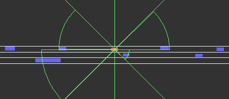
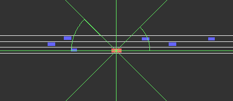
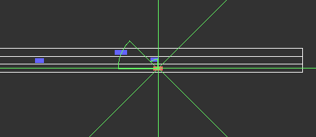
Fig. 6 visualizes the result of the maximum closeness reconstruction of an arbitrary traffic scenario. The red rectangle represents the ego agent and the blue rectangle depicts the other traffic participants. The maximum closeness predictions for each angular region are illustrated in green. Positions and sizes of all traffic participants originate from our dataset, while the maximum closeness is reconstructed by the trained model. The direction of travel is from left to right for all traffic scenarios. We can see that our model can predict the maximum closeness well.

Visualization of traffic scene and the reconstructed maximum closeness for all angular regions. It depicts a multilane road where the direction of travel is from left to right. The ego agent is red, other traffic participants are blue and the predicted angular regions are green.

To understand our learned representations better, we perform Principal Component Analysis (PCA) on the encoder output of the entire test dataset. Using PCA we can identify clusters in the learned representations. PCA derives a low-dimensional feature set from a higher-dimensional feature set while striving to preserve as much information (i.e. variance) as possible.

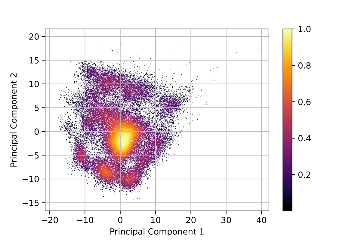
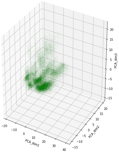
We show the results of \(2D\) PCA decomposition with point density heatmap and 3D PCA decomposition in Fig. 7(a) and Fig. 7(b) respectively. The variance ratio of the three principal components are \(15.17\%\), \(13.69\%\) and \(8.37\%\) respectively. Both 2D PCA and 3D PCA show clear clustering.

| |

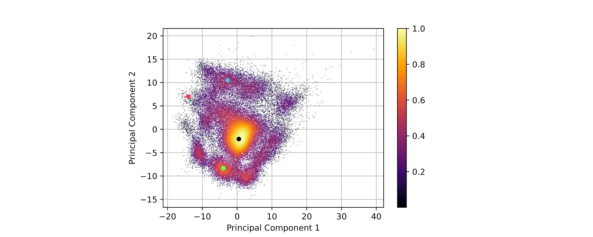
We interpret the PCA results by visualizing traffic scenes at important points of the 2D PCA heatmap. The most common cluster in the 2D PCA heatmap is the cluster around the black dot in Fig. 8, corresponding to the scenario in Fig. 9(b) in which there are close traffic participants around the ego agent. The cluster around the green dot in Fig. 8 is the second most common cluster in the 2D PCA heatmap. This cluster corresponds to scenarios like Fig. 9(a) in which there are fewer close traffic participants around ego agent compared to the main cluster. In addition, we observed that clusters in the heatmap with lower point density correspond to scenarios in which, either there are only a few close traffic participants in front of the ego agent, or behind of the ego agent. One example is illustrated in Fig. 9(d), which corresponds to the red dot in Fig. 8.

We can conclude, that clusters in the learned representations correspond to actual clusters in the surrounding environment from the perspective of the ego agent. It indicates the learned representations contain the latent information from the surrounding environment and can be used as meaningful representations for subsequent reinforcement learning problems.

Conclusion

In this work, we have shown that modeling traffic scenes as graphs and using GNNs to learn representations of these traffic scenes leads to powerful state representations. In future work, we will use our learned representations as the input of reinforcement learning agents for motion planning. The representations can be further improved by extending the reconstruction task to predict the relative angle between the ego agent and the nearest agent in each region. In addition, a sequential model could be developed to predict the closeness between the ego agent and other traffic participants in future timestamps for a better representation.

Appendix

The entire pipeline as described in this paper, detailing how we construct the learned representations from the highD dataset.

Footnotes

1. De Bruin, Tim, et al. “Integrating state representation learning into deep reinforcement learning.” IEEE Robotics and Automation Letters 3.3 (2018): 1394-1401.

2. Goodfellow, Ian, Yoshua Bengio, and Aaron Courville. Deep learning. MIT press, 2016.

3. Gori, Marco, Gabriele Monfardini, and Franco Scarselli. “A new model for learning in graph domains.” Proceedings. 2005 IEEE international joint conference on neural networks. Vol. 2. No. 2005. 2005.

4. Gilmer, Justin, et al. “Neural message passing for quantum chemistry.” International conference on machine learning. PMLR, 2017.

5. Wang, Yue, et al. “Dynamic graph cnn for learning on point clouds.” Acm Transactions On Graphics (tog) 38.5 (2019): 1-12.

6. Chen, Jun, and Haopeng Chen. “Edge-featured graph attention network.” arXiv preprint arXiv:2101.07671 (2021).

7. Veličković, Petar, et al. “Graph attention networks.” arXiv preprint arXiv:1710.10903 (2017).

8. Krajewski, Robert, et al. “The highd dataset: A drone dataset of naturalistic vehicle trajectories on german highways for validation of highly automated driving systems.” 2018 21st International Conference on Intelligent Transportation Systems (ITSC). IEEE, 2018.

9. Fey, Matthias, and Jan Eric Lenssen. “Fast graph representation learning with PyTorch Geometric.” arXiv preprint arXiv:1903.02428 (2019).

10. Althoff, Matthias, Markus Koschi, and Stefanie Manzinger. “CommonRoad: Composable benchmarks for motion planning on roads.” 2017 IEEE Intelligent Vehicles Symposium (IV). IEEE, 2017.

11. Paszke, Adam, et al. “Pytorch: An imperative style, high-performance deep learning library.” Advances in neural information processing systems 32 (2019).